where η = E–E₀ is the overvoltage, I₀ is the exchange current density, n is the number of electrons, F is Faraday's constant, R is the gas constant, T is the temperature, α (0<α<1) is the charge transfer coefficient.
Knowledge of the Tafel slope is essential because it directly reflects the kinetics of the electrocatalytic reaction: it shows how quickly the current increases with the applied overpotential and provides the charge transfer coefficient (α), which is a fingerprint of the reaction mechanism.
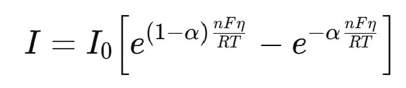
The starting point is the Butler–Volmer equation:
where η = E–E₀ is the overvoltage, I₀ is the exchange current density, n is the number of electrons, F is Faraday's constant, R is the gas constant, T is the temperature, α (0<α<1) is the charge transfer coefficient.
When η is sufficiently large, one exponential component dominates, and this simplifies to the Tafel equation:

where b is the Tafel slope coefficient.
Traditional Tafel analysis requires a visual determination of the ‘linear’ region on the η versus log I plot, manual selection of appropriate limits, and application of often arbitrary corrections for background or mass transfer. Such subjectivity can lead to the significant discrepancies in α and b values between users. To eliminate those ambiguities, Corva et al. developed Differential Tafel Analysis (DTA). By computing the first (dI/dE) and second (d²I/dE²) derivatives of a linear-sweep voltammogram I(E), DTA automatically cancels constant offsets and linear drifts, objectively identifies the pure charge-transfer window (peaking in d²I/dE²), and fits both ln I and ln (dI/dE) over that same window. The result is a robust, user-bias-free determination of α and the Tafel slope.
|
Smoothing (Savitzky–Golay filter) window size:
(d²(Current)/dV²)max at Potential = V. Select potential window size (mV):
Potential (V):
|
Normalized Current (A) vs Potential (V) |
Tafel slope: Potential vs Log10(Current) |
LN(Normalized Current (A)) vs Potential (V) |